AI Super-Resolution Algorithm User Guide

Nissho Technology Co., Ltd.
http://www.dragonwake.com
info@dragonwake.com
Created: 2026/06/20

This tutorial explains ONNX/RKNN conversion for the XLSR super-resolution model and deployment on the CSUN RV1126B board.

copyright@2026 Nissho Technology Co., Ltd.

Revision History

No.	Version	Description	Date
1	Ver1.0	Initial release	2026/06/20

The information in this document may be changed without prior notice for document improvement. Please refer to our website for the latest version.
https://www.dragonwake.com

Reproduction of this document in any form is strictly prohibited without the written permission of Nissho Technology Co., Ltd.

1. XLSR Overview

XLSR is an image super-resolution algorithm designed for the 2021 Mobile AI Real-Time Single Image Super-Resolution Challenge. By combining an efficient mobile network module design with a quantization-robust training strategy that considers hardware characteristics, XLSR provides excellent reconstruction quality, a very small number of parameters, and real-time performance on mobile devices. It won the challenge. The quality metrics of XLSR are PSNR 29.58 and SSIM 0.86.

1.1 Model Export Optimization

To emphasize image details after super-resolution, a Laplacian operator layer, SharpeningLayer(), is added to the final layer of the original model. The Laplacian kernel is adjustable. In addition, to avoid transposing output data from NCHW to NHWC during RKNN model post-processing, a transpose layer is added at the end of the model forward computation to improve speed.

Run export_onnx.py on the PC side to convert the PT model to ONNX.

The main code example for ONNX export is shown below.

from model.models import *
import torch

h, w = 360, 640
scaling_factor = 2  # 2 or 4
weight = r"weight/xlsr_2x_checkpoint_float32.pth.tar"
output_file = r"weight/xlsr_{}x_{}x{}.onnx".format(scaling_factor, h, w)
model = XLSRRelease(scaling_factor=scaling_factor)
checkpoint = torch.load(weight, map_location='cpu', weights_only=False)
model.load_state_dict(checkpoint["state_dict"], strict=False)
model.eval()
input_size = (3, h, w)  # c, h, w
example_input = torch.randn((1,) + input_size, requires_grad=False)
torch_out = torch.onnx.export(
    model,
    example_input,
    output_file,
    export_params=True,
    input_names=["image"],
    output_names=["upscaled_image"],
    opset_version=11
)
print("export finish")

2. Downloading Materials

Download the materials and source code required for this manual from the following links.

1. Training source code GitHub: https://github.com/csunltd/rv1126b-yolov5
2. Other source code: AIDemo_uhr_All.zip

The extracted directory structure is shown below.

|-- 03-model_convert      Source code for AI model conversion
|-- 04-AI_deploy          Source code for AI model deployment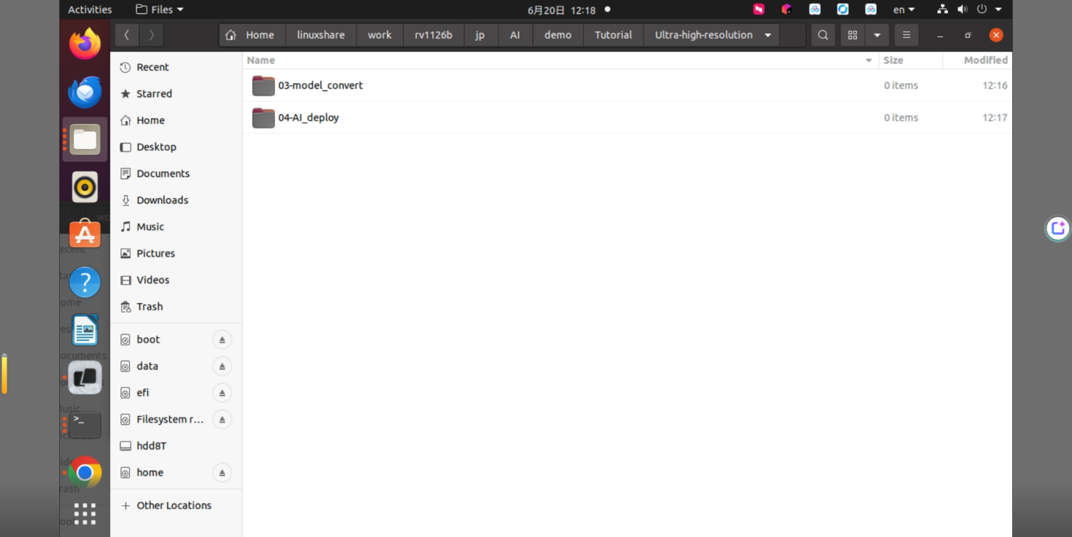

Figure 2-1. Directory structure after extracting the Ultra-high-resolution package

3. rknn-toolkit Model Conversion

3.1 Building the rknn-toolkit Model Conversion Environment

To run an ONNX model on the CSUN RV1126B board, it must be converted to an RKNN model. Therefore, build the rknn-toolkit model conversion tool environment in advance. TensorFlow, TensorFlow Lite, Caffe, Darknet, and other models can also be converted through a similar process. This tutorial uses an ONNX model as an example.

For the environment setup procedure, refer to the AI Model Conversion Environment Setup Guide.

3.2 Converting an ONNX Model to an RKNN Model

This document supports evaluation and execution of models with the .rknn extension. Common trained models from TensorFlow, TensorFlow Lite, Caffe, Darknet, ONNX, PyTorch, and other frameworks can be converted to RKNN models using the provided RKNN-Toolkit2. Models trained in other frameworks can also be converted to ONNX first, then converted to RKNN.

For detailed conversion steps, refer to the RKNN Model Conversion Tutorial Example.

3.2.1 Extracting the Model Conversion Files

After downloading and extracting the model conversion demo from the materials section, run the following commands.

cd /data/project/sales/csun/rv1126b/jp/AI/demo/Tutorial/Ultra-high-resolution/03-model_convert
tar -xvf xlsr-python-2x.tar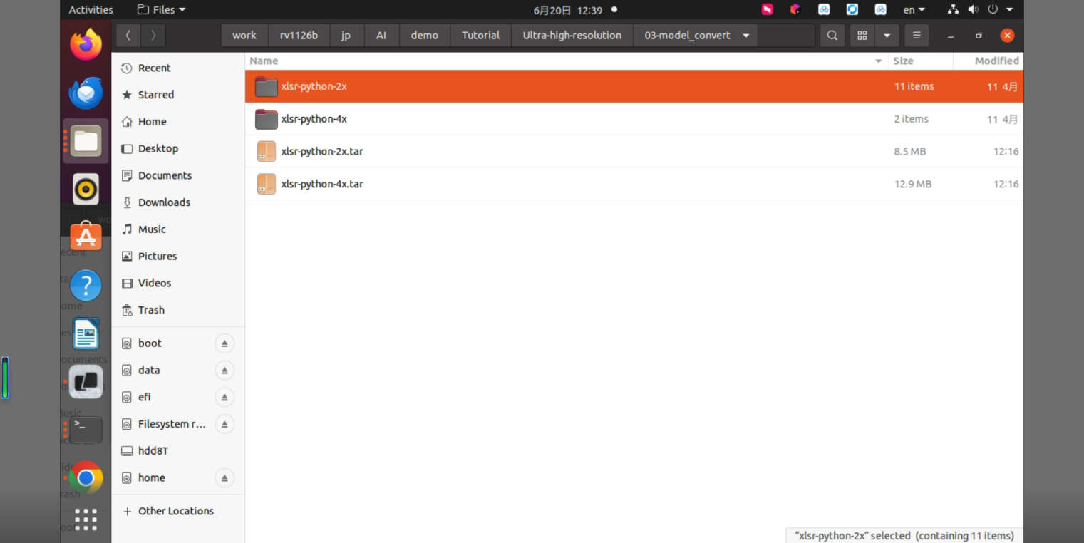

Figure 3-1. Command for extracting xlsr-python-2x.tar

3.2.2 Entering the Model Conversion Docker Environment

Use the following command to mount the working directory into the Docker image. /data/project/sales/csun/rv1126b/jp/AI/demo/Tutorial is used as the working directory and mapped to /test inside the container. /dev/bus/usb:/dev/bus/usb mounts USB devices into the container.

docker run -t -i --privileged   -v /dev/bus/usb:/dev/bus/usb   -v /data/project/sales/csun/rv1126b/jp/AI/demo/Tutorial:/test   rknn-toolkit2:2.3.2-cp38 /bin/bash

Figure 3-2. Command for starting the RKNN-Toolkit2 Docker environment

3.2.3 Generating the Quantization Image List

Inside the Docker environment, move to the model conversion working directory.

cd /test/Ultra-high-resolution/03-model_convert/xlsr-python-2x

Figure 3-3. Moving to the XLSR model conversion working directory

Run gen_datas.py to generate the quantization image list.

python gen_datas.py

Figure 3-4. Running the quantization image list generation script

The generated quantization image list is saved as datas_360x640.txt.

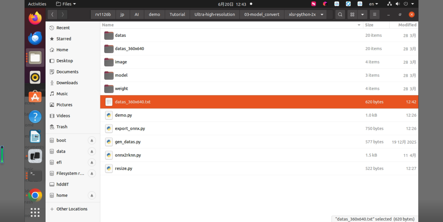
Figure 3-5. Confirming the generated datas_360x640.txt file

3.2.4 Converting the ONNX Model to an RKNN Model

By default, the onnx2rknn.py script uses do_quant = False, which disables quantization. To use INT8 quantization, change it to do_quant = True. The main settings include input resolution, quantization type, target platform, ONNX input model, RKNN output path, and quantization dataset list.

from rknn.api import RKNN

if __name__ == '__main__':
    h, w = 360, 640
    do_quant = True

    quant = "fp16"
    if do_quant:
        quant = "int8"
    platform = "rv1126b"
    model_path = r"weight/xlsr_2x_{}x{}.onnx".format(h, w)
    output_path = r"weight/xlsr_2x_{}x{}-{}.rknn".format(h, w, quant)
    data_set = r'datas_{}x{}.txt'.format(h, w)

    # Create RKNN object
    rknn = RKNN(verbose=False)

    # Pre-process config
    print('--> Config model')
    rknn.config(mean_values=[[0, 0, 0]],
                std_values=[[255, 255, 255]],
                target_platform=platform,
                optimization_level=3,
                model_pruning=True,
                compress_weight=True,
                # sparse_infer=True,
                output_optimize=True,
                custom_string='output_format=nhwc',
                )
    print('done')

    # Load model
    print('--> Loading model')
    ret = rknn.load_onnx(model=model_path, inputs=['image'], input_size_list=[[1, 3, h, w]])
    if ret != 0:
        print('Load model failed!')
        exit(ret)
    print('done')

    # Build model
    print('--> Building model')
    ret = rknn.build(do_quantization=do_quant, dataset=data_set)
    if ret != 0:
        print('Build model failed!')
        exit(ret)
    print('done')

    # Export rknn model
    print('--> Export rknn model')
    ret = rknn.export_rknn(output_path)
    if ret != 0:
        print('Export rknn model failed!')
        exit(ret)
    print('done')

Run the following command to convert the model.

python onnx2rknn.py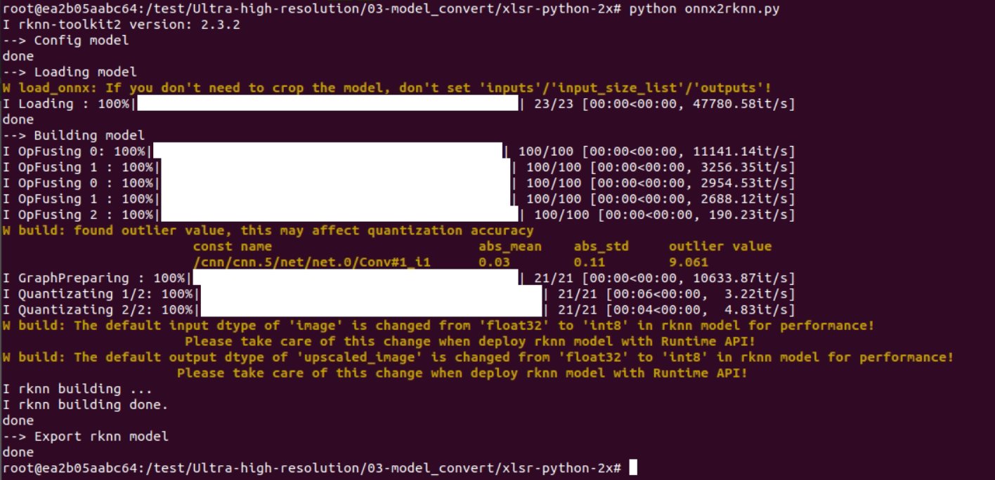

Figure 3-6. ONNX to RKNN model conversion result

The generated model is saved to output_path and can be executed in the RKNN environment and on the CSUN RV1126B board.

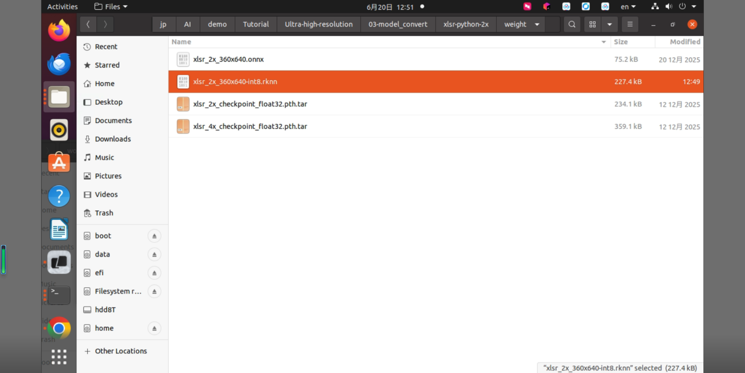
Figure 3-7. RKNN model file generated after conversion

4. XLSR Model Deployment

4.1 Model Deployment Description

This section describes the procedure for deploying the XLSR model to the CSUN RV1126B board. The xlsr_2x_360x640-int8.rknn model used in this chapter is a 2x upscaling model converted from the official xlsr_2x_checkpoint_float32.pth.tar model.

4.2 Preparation

4.2.1 Hardware Preparation

Prepare the RV1126B board, a Type-C data cable, and a LAN cable. Log in to the RV1126B board through SSH using MobaXterm. For details, refer to the Getting Started Guide.

Connect using a LAN cable.

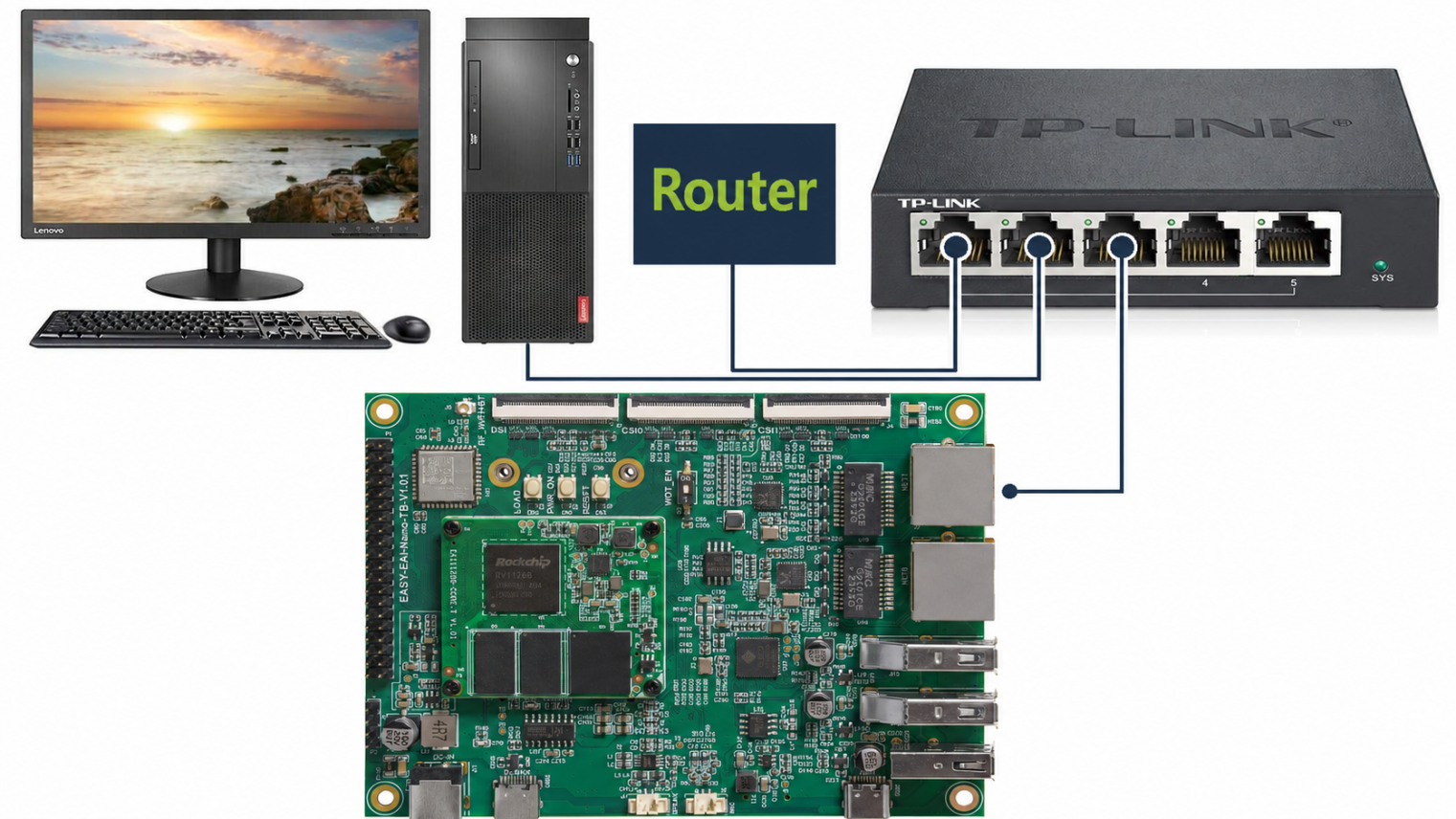
Figure 4-1. LAN connection topology between the RV1126B board and PC

Connect using a serial cable, Type-C.

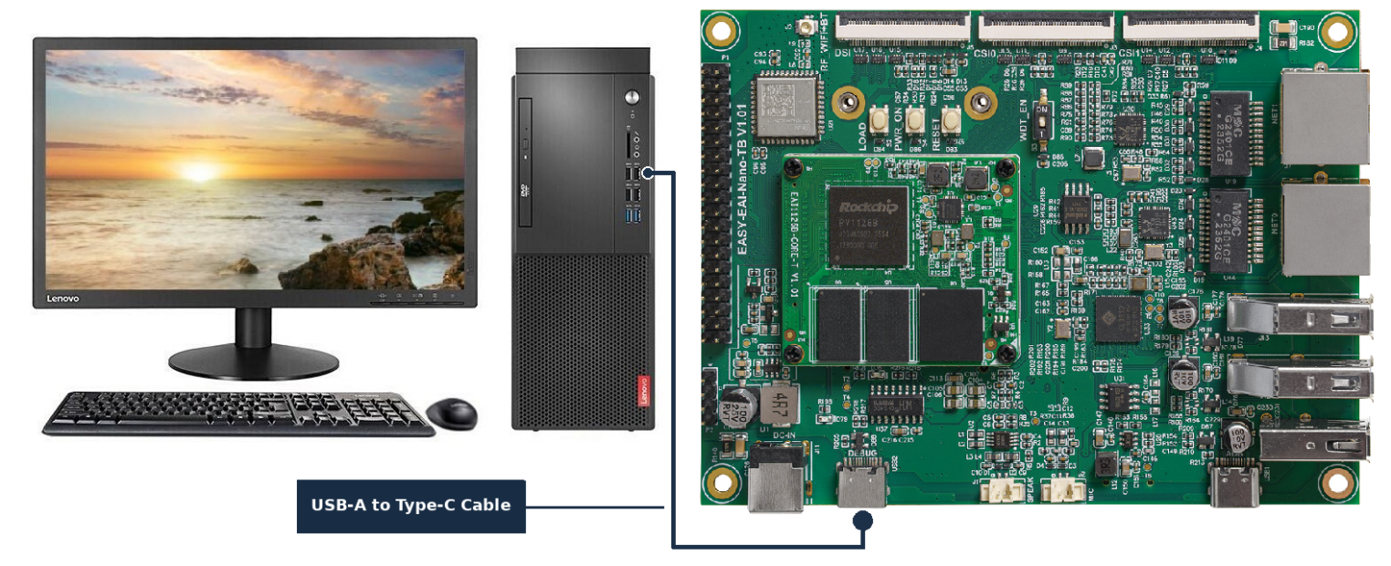
Figure 4-2. Type-C serial connection topology

4.2.2 Preparing the Development Environment

If this is your first time reading this document, refer to the Getting Started Guide and build the compilation environment by following the described procedure.

On the Ubuntu system of the PC, run the run script to enter the RV1126B compilation environment.

cd ~/develop_environment
./run.sh 2204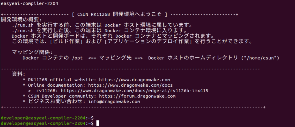

Figure 4-3. Starting the RV1126B Docker development environment

4.3 Building the Sample Program

After moving the downloaded package to the RV1126B Docker development environment, run the following commands to extract it.

cd /opt/linuxshare/work/rv1126b/jp/AI/demo/Tutorial/Ultra-high-resolution/04-AI_deploy
tar -xvf SuperResolution.tar

The structure after download and extraction is shown below.

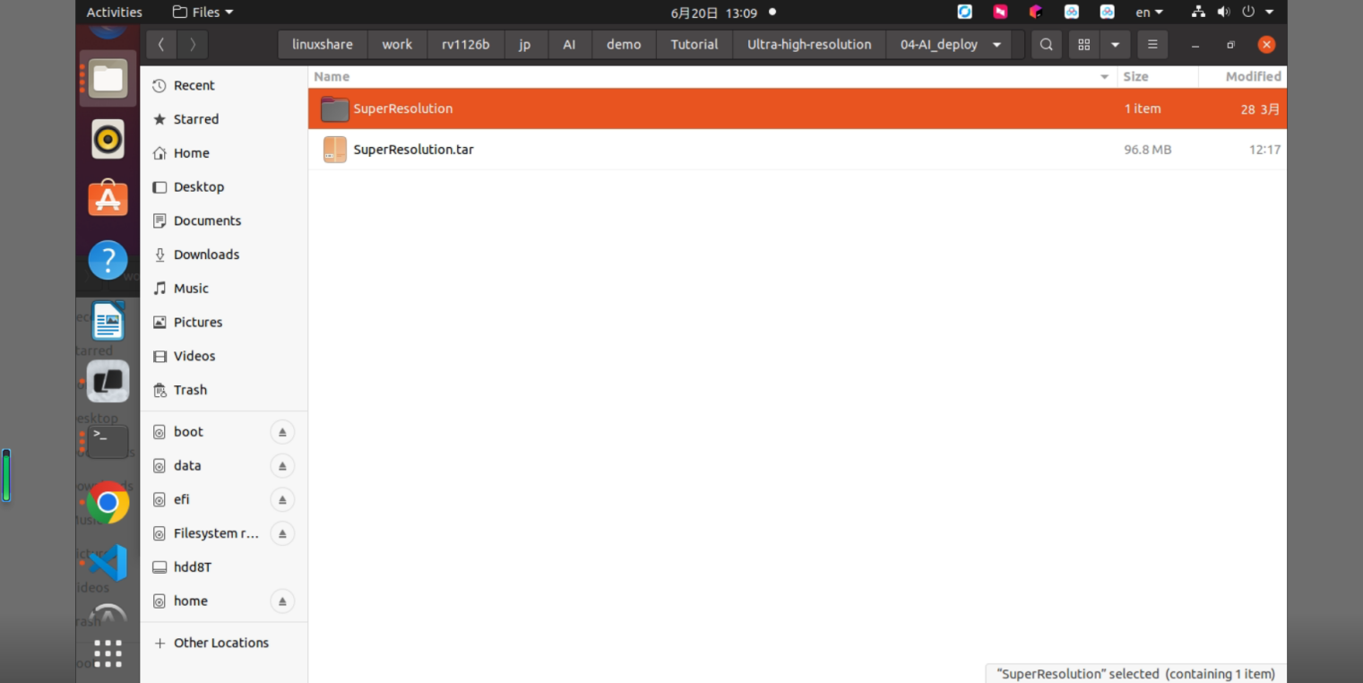
Figure 4-4. Directory structure after extracting the SuperResolution source code

In this tutorial, the source code is compiled directly on the board. First transfer the extracted source code to the board with the following command.

scp -r SuperResolution nano@192.168.10.85:/userdata

After the transfer, connect to the CSUN RV1126B board through SSH and compile with the following commands.

ssh nano@192.168.10.85

cd /userdata/SuperResolution
mkdir build
cd build
cmake ..
make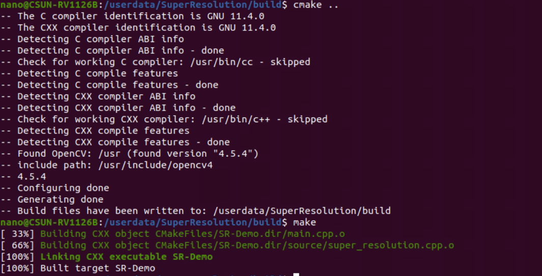

Figure 4-5. Build result of the SuperResolution sample program

If the following error message appears during compilation, install libopencv-dev.

CMAKE_MODULE_PATH this project has asked CMake to find a package configuration file provided by "OpenCV", but CMake did not find one.

sudo apt-get update
sudo apt-get install libopencv-dev

4.4 Running the XLSR Model on the Development Board

After compilation, run the following command.

./SR-Demo ../model/xlsr_2x_360x640-int8.rknn ../image/SRC-360P.jpg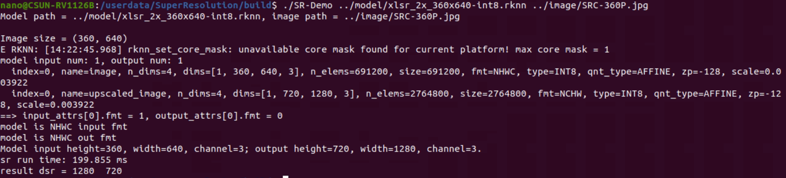

Figure 4-6. XLSR model execution result using SR-Demo

The original 720P image is shown below.

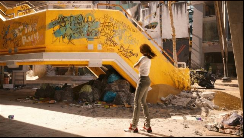
Figure 4-7. Original 720P image

The AI super-resolution result is shown below.

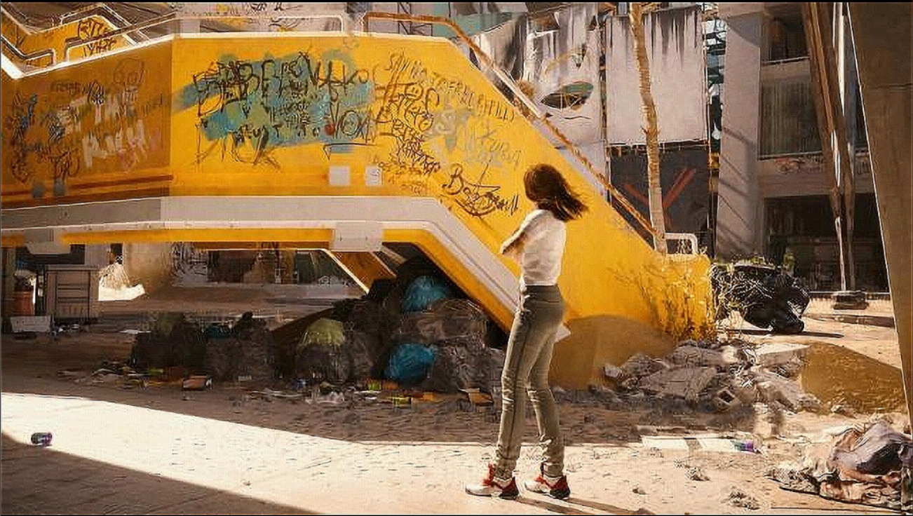
Figure 4-8. AI super-resolution output image