YOLOv11 Training and Deployment Guide

Document Information

This tutorial describes how to train a YOLOv11 object detection model and deploy it to the CSUN RV1126B board.

Item	Description
Document name	YOLOv11 Training and Deployment Guide
Company	Nissho Technology Co., Ltd.
URL	http://www.dragonwake.com
E-mail	info@dragonwake.com
Created date	2026/06/06
Version	Ver1.0
Revision	Initial creation

Revision History

No.	Version	Revision	Date
1	Ver1.0	Initial creation	2026/06/06

The information in this document may be changed without prior notice for documentation improvement. Refer to the company website for the latest version.

Reproduction of this document in any form without written permission from Nissho Technology Co., Ltd. is strictly prohibited.

1. YOLOv11 Overview

The YOLO11 series is a newer, lightweight, and efficient model family in the YOLO lineup. It provides strong detection performance and follows the design direction of the YOLO series developed by Ultralytics, the team that released YOLOv8.

This guide explains how to train the YOLO11 object detection algorithm and deploy it to the CSUN RV1126B board. Refer to previously published documents for data annotation methods.

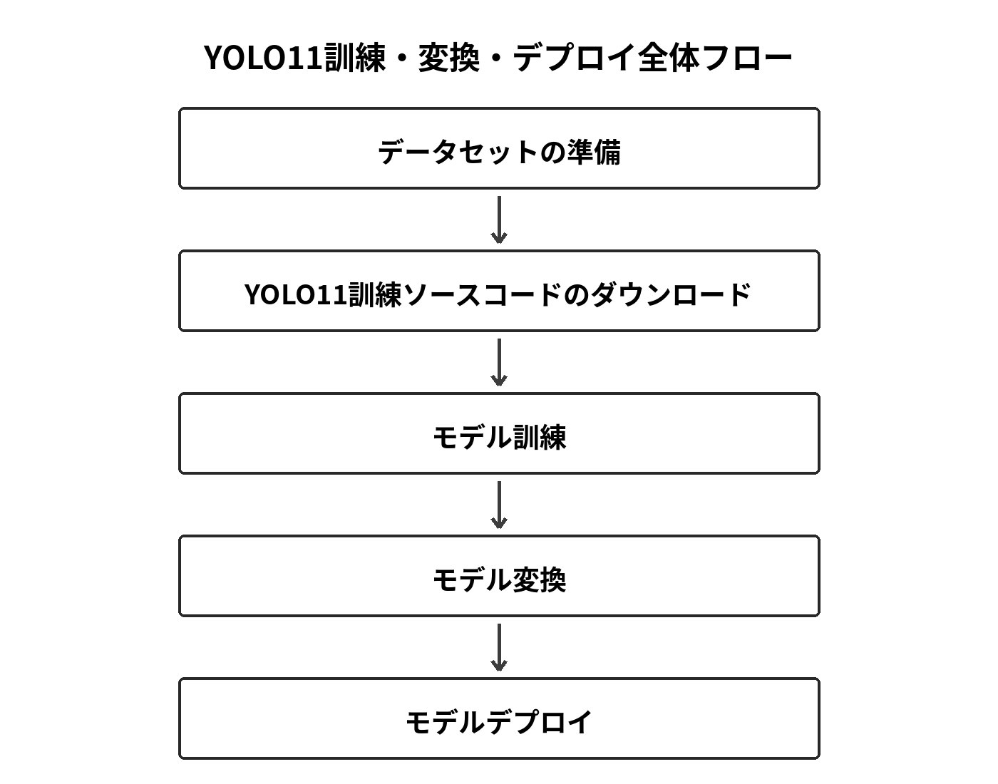
Figure1-1 Overall YOLOv11 training, conversion, and deployment workflow from dataset preparation to training, model conversion, and deployment.

2. Download Materials

Download the required materials and source code from the following link:

https://dl.dragonwake.com/download/rv1126b/AI/demo/yolov11/AIDemo_yolov11_All.zip

The extracted package contains the following main directories:

|-- 01-data          Dataset
|-- 02-training      Source code for training
|-- 03-model_convert Source code for AI model conversion
|-- 04-AI_deploy     Source code for AI model deployment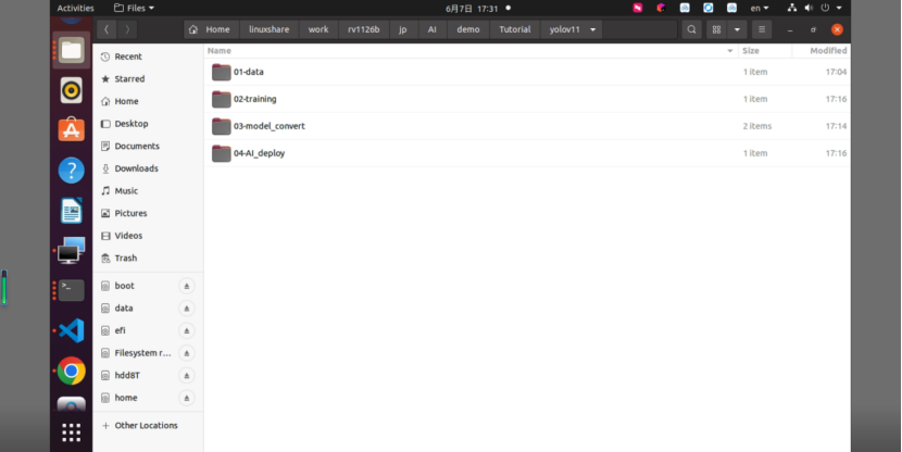

Figure2-1 Directory structure after extracting AIDemo_yolov11_All.zip.

3. Training the YOLOv11 Object Detection Algorithm

The YOLOv11 training source code includes changes in the export section compared with the original Ultralytics GitHub version. Therefore, use the training source code provided with this package.

3.1 Prepare the Dataset

Before starting YOLO11 training, prepare a training dataset such as VOC2007.

http://host.robots.ox.ac.uk/pascal/VOC/voc2007/index.html

This guide places the original VOC2007 dataset under the 01-data directory. The VOC2007 train.txt file is used for the training set, and val.txt is used for the validation set.

mkdir -p /opt/linuxshare/work/rv1126b/jp/AI/demo/Tutorial/yolov11/01-data
cd /opt/linuxshare/work/rv1126b/jp/AI/demo/Tutorial/yolov11/01-data
wget https://www.robots.ox.ac.uk/~vgg/data/pascal/VOC/voc2007/VOCtrainval_06-Nov-2007.tar
tar -xf VOCtrainval_06-Nov-2007.tar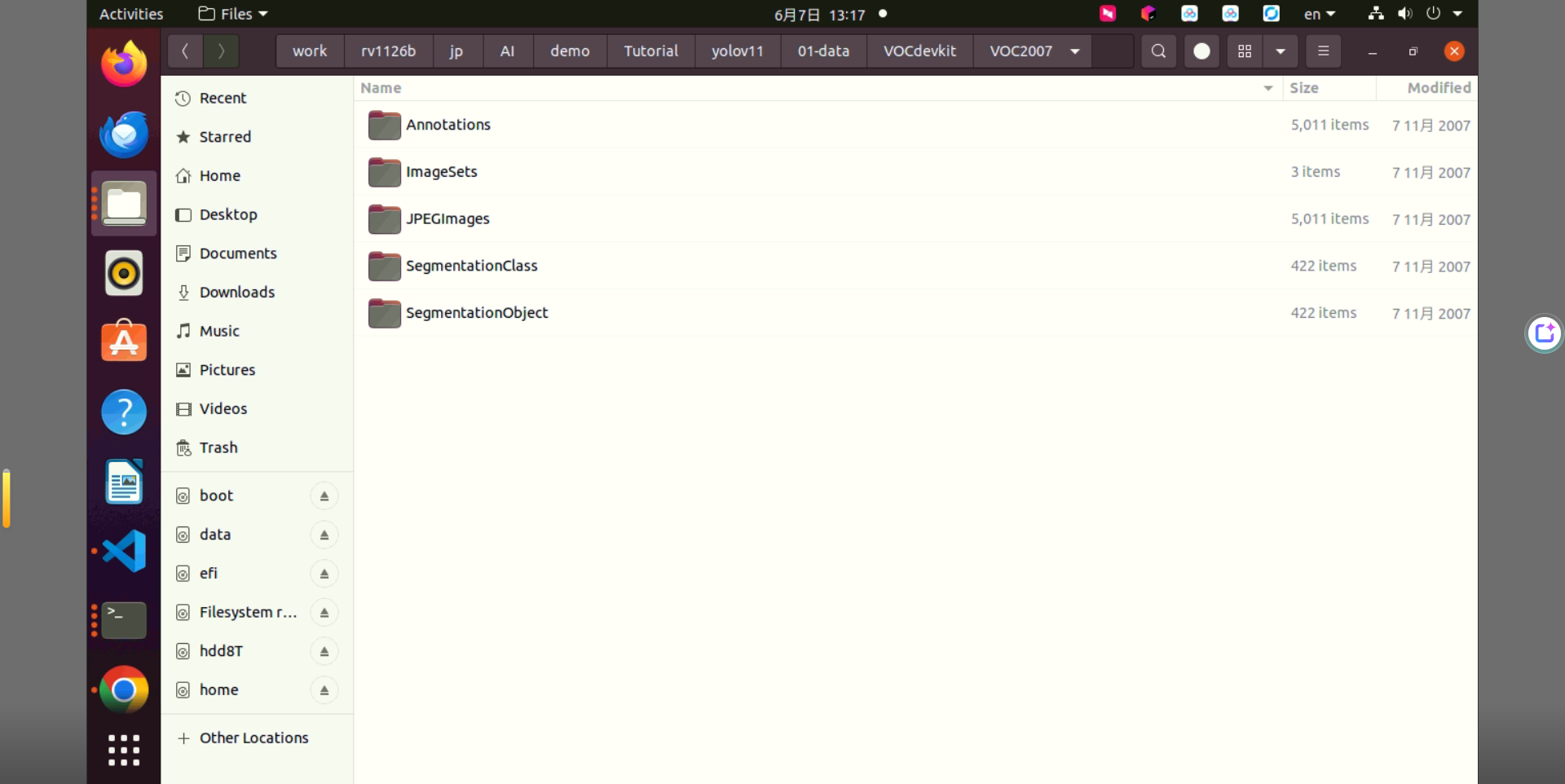

Figure3-1 Directory structure after extracting the VOC2007 dataset.

3.2 Convert VOC to YOLO Format

After preparing the data, use data/voc_2_yolo.py to convert VOC-format annotations into YOLO format. The converted data is saved in the yolo_datas directory at the same hierarchy as the source data.

cd /opt/linuxshare/work/rv1126b/jp/AI/demo/Tutorial/yolov11/02-training/ultralytics_yolo11
rm -rf demo/voc2007/datas/yolo_datas
python data/voc_2_yolo.py

3.3 Configure Training Parameters

After data conversion, configure data.yaml, default.yaml, and yolo11.yaml for model training.

File	Description
data.yaml	Specifies training/validation data paths, class count, and class names.
default.yaml	Specifies YOLO11 training parameters and can be adjusted as needed.
yolo11.yaml	Defines the YOLO11 model architecture. The class count must be modified for the dataset.

3.4 Train the Model

After completing the preceding steps, open train.py and set the paths to data.yaml, default.yaml, and yolo11.yaml.

from ultralytics import YOLO
import os

# OMP 関連エラー（例: "OMP: Hint This means..."）が発生する場合に使用します。
os.environ["KMP_DUPLICATE_LIB_OK"] = "TRUE"

if __name__ == '__main__':
    # 学習設定ファイル、データセット設定ファイル、モデル構造ファイルを指定します。
    # 本スクリプトは ultralytics_yolo11 のプロジェクトルートで実行してください。
    cfg = "./demo/voc2007/cfg/default.yaml"
    data = "./demo/voc2007/cfg/data.yaml"
    weight = "./demo/voc2007/cfg/yolo11.yaml"  # .pt または yolo11.yaml を指定できます。

    print("YOLO11 物体検出モデルの学習を開始します。")
    print(f"学習設定ファイル: {cfg}")
    print(f"データセット設定ファイル: {data}")
    print(f"モデルファイル: {weight}")

    model = YOLO(weight)
    results = model.train(
        data=data,
        cfg=cfg
    )

    print("YOLO11 物体検出モデルの学習が完了しました。")

Run the following commands in the RV1126B Docker development environment to start training:

cd /home/csun/linuxshare/work/rv1126b/jp/embedded/images/develop_environment
./run.sh 2204
cd /opt/linuxshare/work/rv1126b/jp/AI/demo/Tutorial/yolov11/02-training/ultralytics_yolo11
python train.py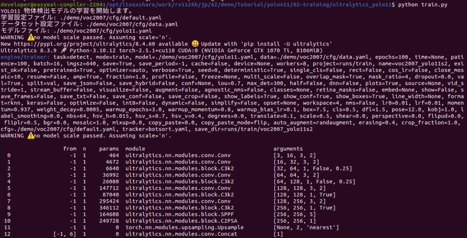

Figure3-2 Model structure and training log shown when YOLOv11 training starts.

The output after training completes is shown below.

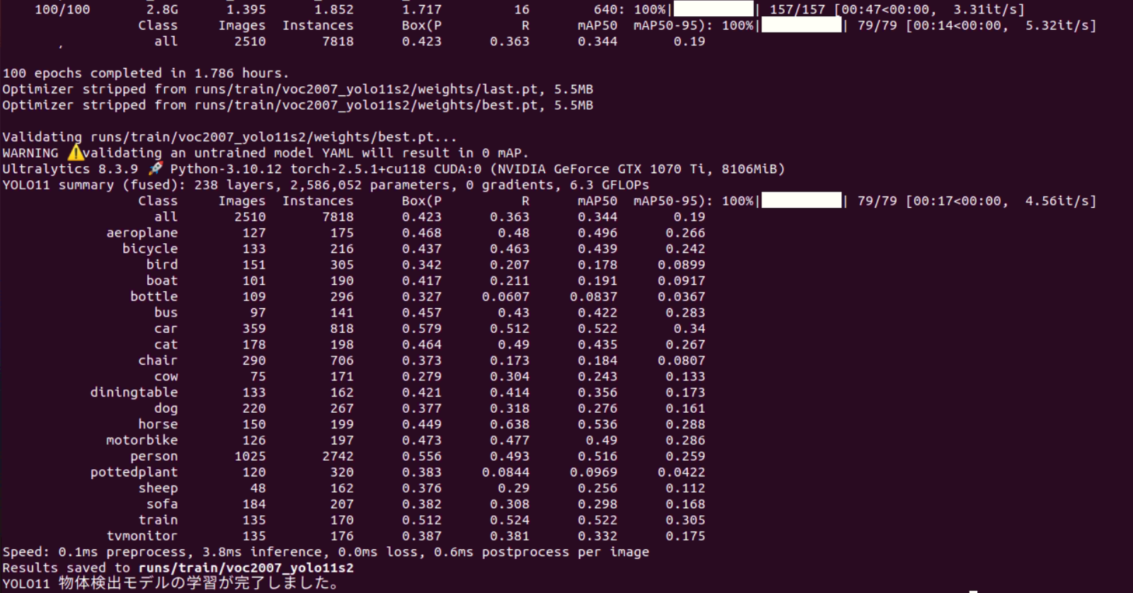
Figure3-3 Validation results displayed after YOLOv11 training completes.

Note: The training procedure in this document is a sample for workflow demonstration. Subsequent inference and model conversion use the standard YOLOv11 80-class model.

The generated model file is:

./runs/train/voc2007_yolo11s2/weights/best.pt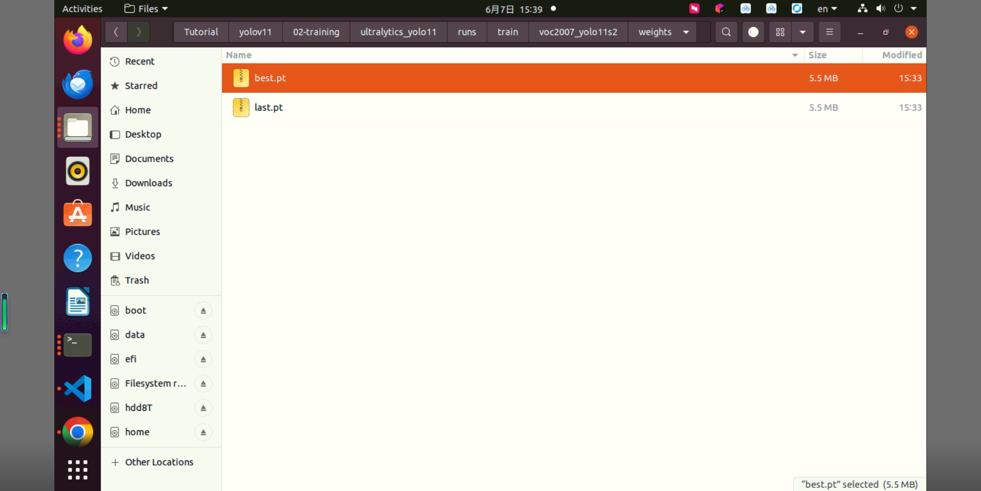

Figure3-4 Output directory containing best.pt and last.pt after training.

3.5 Model Inference on the PC

After training completes, the training process and the best validation model are saved in the project directory configured in default.yaml. Run predict.py to perform an initial check of the model behavior.

predict.py sets the model path, input image, inference device, and image size, then performs image preprocessing, model inference, and result drawing. Confirm the actual model file path before running it.

if __name__ == '__main__':
    random.seed(0)
    device_ = "cpu"
    imgsz = (640, 640)

    # 学習済みモデルと推論画像を指定します。
    # 本スクリプトは ultralytics_yolo11 のプロジェクトルートで実行してください。
    model_path = "./runs/train/voc2007_yolo11s2/weights/best.pt"
    img_path = "./demo/images/bus.jpg"
    is_dir = os.path.isdir(img_path)

    print("YOLO11 モデルの推論を開始します。")
    print(f"使用デバイス: {device_}")
    print(f"入力モデル: {model_path}")
    print(f"入力画像パス: {img_path}")

    device = select_device(device_)
    model = YOLO(model_path)

    # モデル推論を実行し、結果画像を入力画像と同じディレクトリへ保存します。
    # 単一画像を指定した場合は result.jpg として保存します。

Run the following command:

python predict.py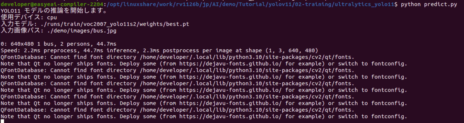

Figure3-5 Inference log generated by predict.py.

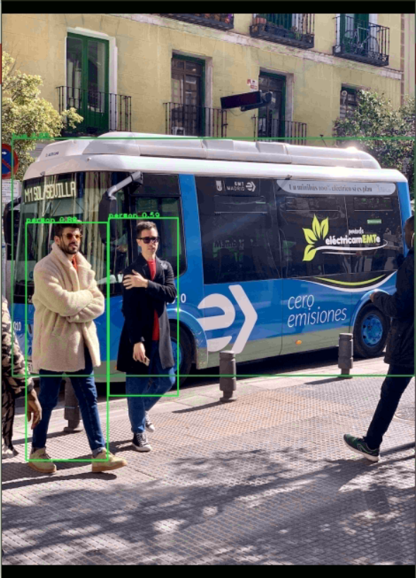
Figure3-6 Object detection result image produced by YOLOv11 on the PC side.

3.6 Convert the PT Model to ONNX

Run export.py on the PC side to export the PT model to ONNX or a format used for RKNN conversion. The example code specifies format = 'rknn'.

from ultralytics import YOLO

if __name__ == '__main__':
    # エクスポート形式を指定します。
    # 本プロジェクトの YOLO11 では、RKNN 変換用に rknn 形式を指定します。
    # 選択可能な形式例: 'torchscript', 'onnx', 'openvino', 'engine', 'coreml',
    # 'saved_model', 'pb', 'tflite', 'edgetpu', 'tfjs', 'paddle', 'ncnn', 'rknn'
    format = 'rknn'

    # 学習済みモデルを指定します。
    # default.yaml の project が voc2007 の場合、通常は以下のパスに best.pt が保存されます。
    # 必要に応じて、実際の学習結果ディレクトリに合わせて変更してください。
    weight = "./runs/train/voc2007_yolo11s2/weights/best.pt"  # .pt または yolo11.yaml を指定できます。

    print("YOLO11 モデルのエクスポートを開始します。")
    print(f"入力モデル: {weight}")
    print(f"エクスポート形式: {format}")

    model = YOLO(weight)
    results = model.export(format=format)

    print("YOLO11 モデルのエクスポートが完了しました。")

Run the following command:

python export.py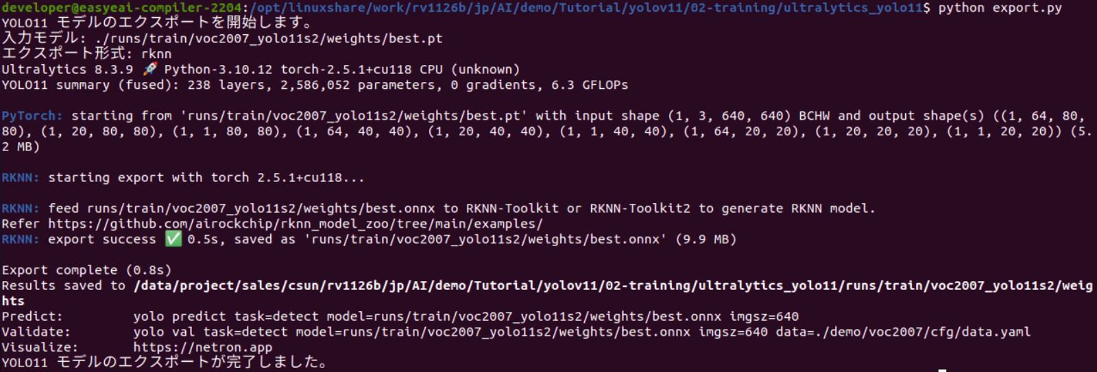

Figure3-7 Terminal log generated when export.py exports the PT model.

The converted model file is saved in the same directory.

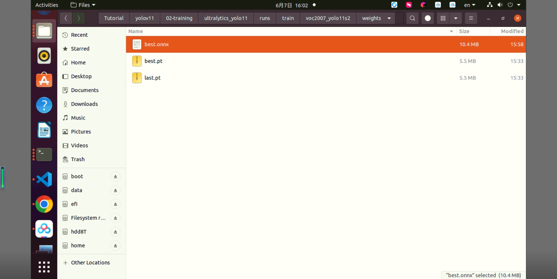
Figure3-8 Directory containing the exported ONNX model file.

4. rknn-toolkit Model Conversion

4.1 Build the rknn-toolkit Model Conversion Environment

To run an ONNX model on the CSUN RV1126B board, it must be converted to an RKNN model. Therefore, prepare the rknn-toolkit model conversion environment in advance. TensorFlow, TensorFlow Lite, Caffe, and Darknet models can be converted using a similar flow. This tutorial uses an ONNX model as the example.

Refer to the AI Model Conversion Environment Setup Guide for environment setup steps.

4.2 Convert the ONNX Model to an RKNN Model

Models with the .rknn extension are used for model evaluation and board-side execution. Common models such as TensorFlow, TensorFlow Lite, Caffe, Darknet, ONNX, and PyTorch can be converted to RKNN using RKNN-Toolkit2. Models trained with other frameworks can also be converted to ONNX first and then converted to RKNN.

Refer to the RKNN Model Conversion Tutorial Example for detailed conversion steps.

4.2.1 Extract the Model Conversion Demo

Download the model conversion demo from the materials described in Section 2, then extract it as follows:

cd /data/project/sales/csun/rv1126b/jp/AI/demo/Tutorial/yolov11/03-model_convert
unzip quant_dataset.zip
tar -xJf yolov11_model_convert.tar.xz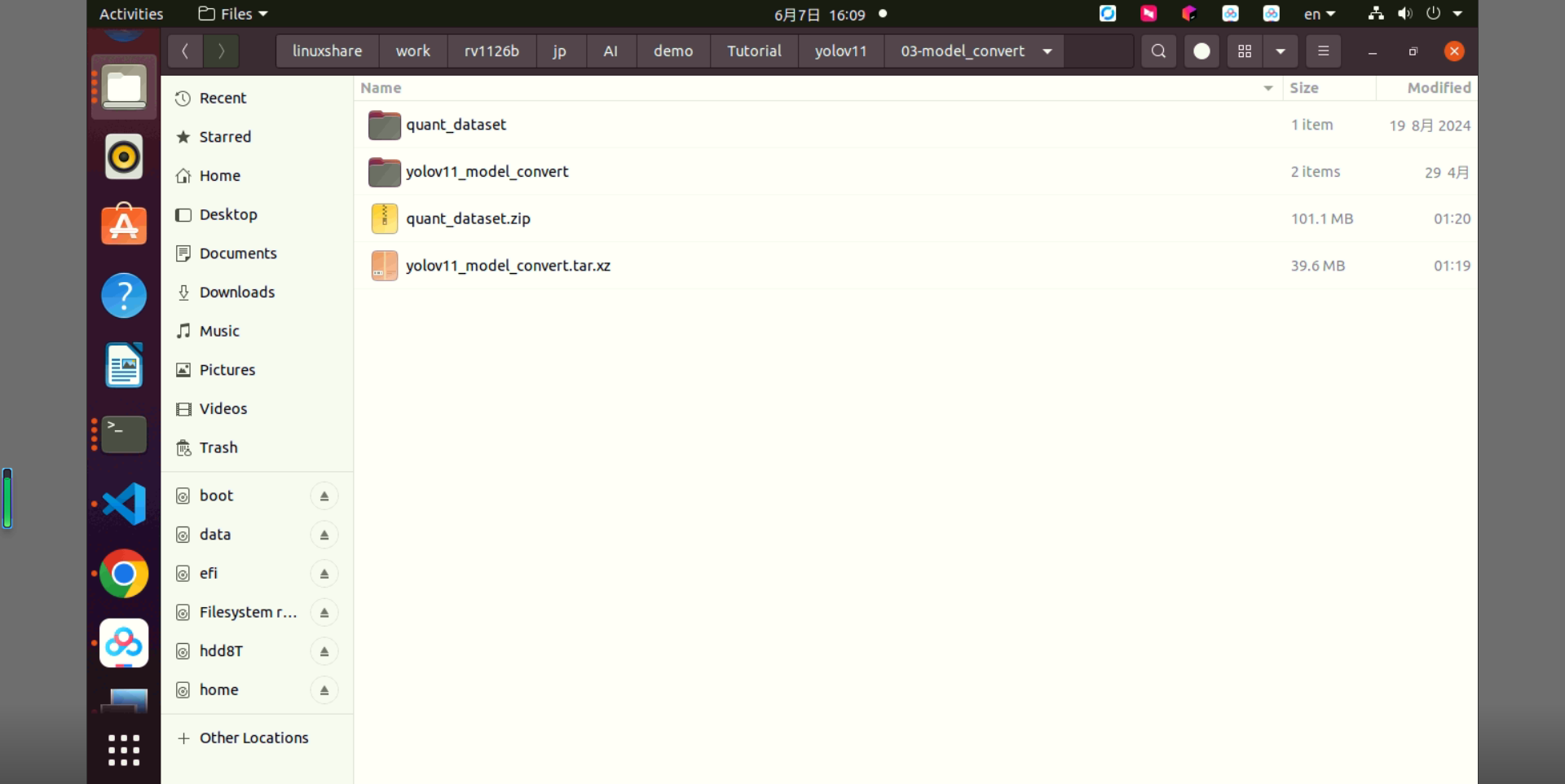

Figure4-1 File structure after extracting the model conversion demo.

4.2.2 Enter the Model Conversion Docker Environment

Use the following command to mount the working directory into the Docker image. /data/project/sales/csun/rv1126b/jp/AI/demo/Tutorial is mapped to /test in the container, and /dev/bus/usb:/dev/bus/usb mounts the USB device path.

docker run -t -i --privileged   -v /dev/bus/usb:/dev/bus/usb   -v /data/project/sales/csun/rv1126b/jp/AI/demo/Tutorial:/test   rknn-toolkit2:2.3.2-cp38 /bin/bash

Figure4-2 Terminal state after entering the RKNN-Toolkit2 Docker environment.

4.2.3 Generate the Quantization Image List

In the Docker environment, enter the model conversion work directory.

cd /test/yolov11/03-model_convert/yolov11_model_convert

Run gen_list.py to generate the quantization image list.

python gen_list.py

Figure4-3 Terminal log after running gen_list.py to generate the quantization image list.

The generated quantization image list is saved as pic_path.txt.

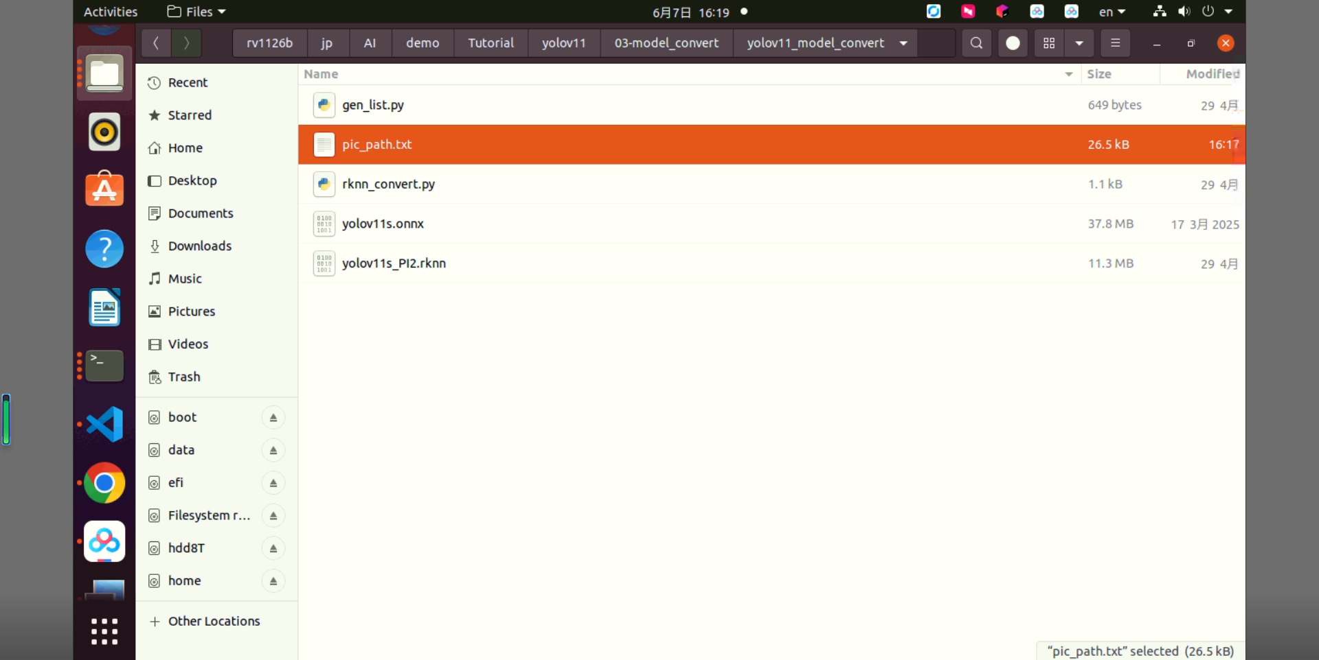
Figure4-4 Location of the generated pic_path.txt file.

4.2.4 Convert the ONNX Model to an RKNN Model

rknn_convert.py performs int8 quantization by default. The main script is shown below.

import sys
from rknn.api import RKNN

# ONNX_MODEL = 'best.onnx'
ONNX_MODEL = 'yolov11s.onnx'
DATASET = './pic_path.txt'
RKNN_MODEL = './yolov11s_rv1126b.rknn'
# RKNN_MODEL = './dog_rope.rknn'
QUANTIZE_ON = True

if __name__ == '__main__':
    # RKNN オブジェクトを作成します。
    rknn = RKNN(verbose=False)

    print('--> Config model')
    rknn.config(mean_values=[[0, 0, 0]], std_values=[[255, 255, 255]], target_platform='rv1126b')
    print('done')

    print('--> Loading model')
    ret = rknn.load_onnx(model=ONNX_MODEL)
    if ret != 0:
        print('Load model failed!')
        exit(ret)
    print('done')

    print('--> Building model')
    ret = rknn.build(do_quantization=QUANTIZE_ON, dataset=DATASET)
    if ret != 0:
        print('Build model failed!')
        exit(ret)
    print('done')

    print('--> Export rknn model')
    ret = rknn.export_rknn(RKNN_MODEL)
    if ret != 0:
        print('Export rknn model failed!')
        exit(ret)
    print('done')

    rknn.release()

Rename best.onnx to yolov11s.onnx, place it in the yolov11_model_convert directory, and run the conversion command below.

cp ../../02-training/ultralytics_yolo11/runs/train/voc2007_yolo11s2/weights/best.onnx yolov11s.onnx
python rknn_convert.py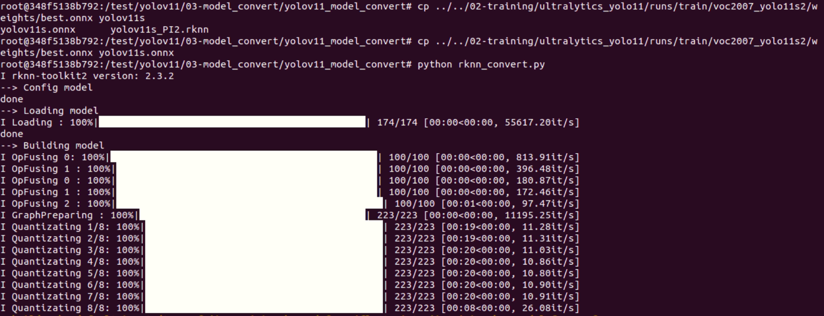

Figure4-5 RKNN conversion log generated by rknn_convert.py.

After successful conversion, an RKNN model that can run on the CSUN RV1126B board is generated.

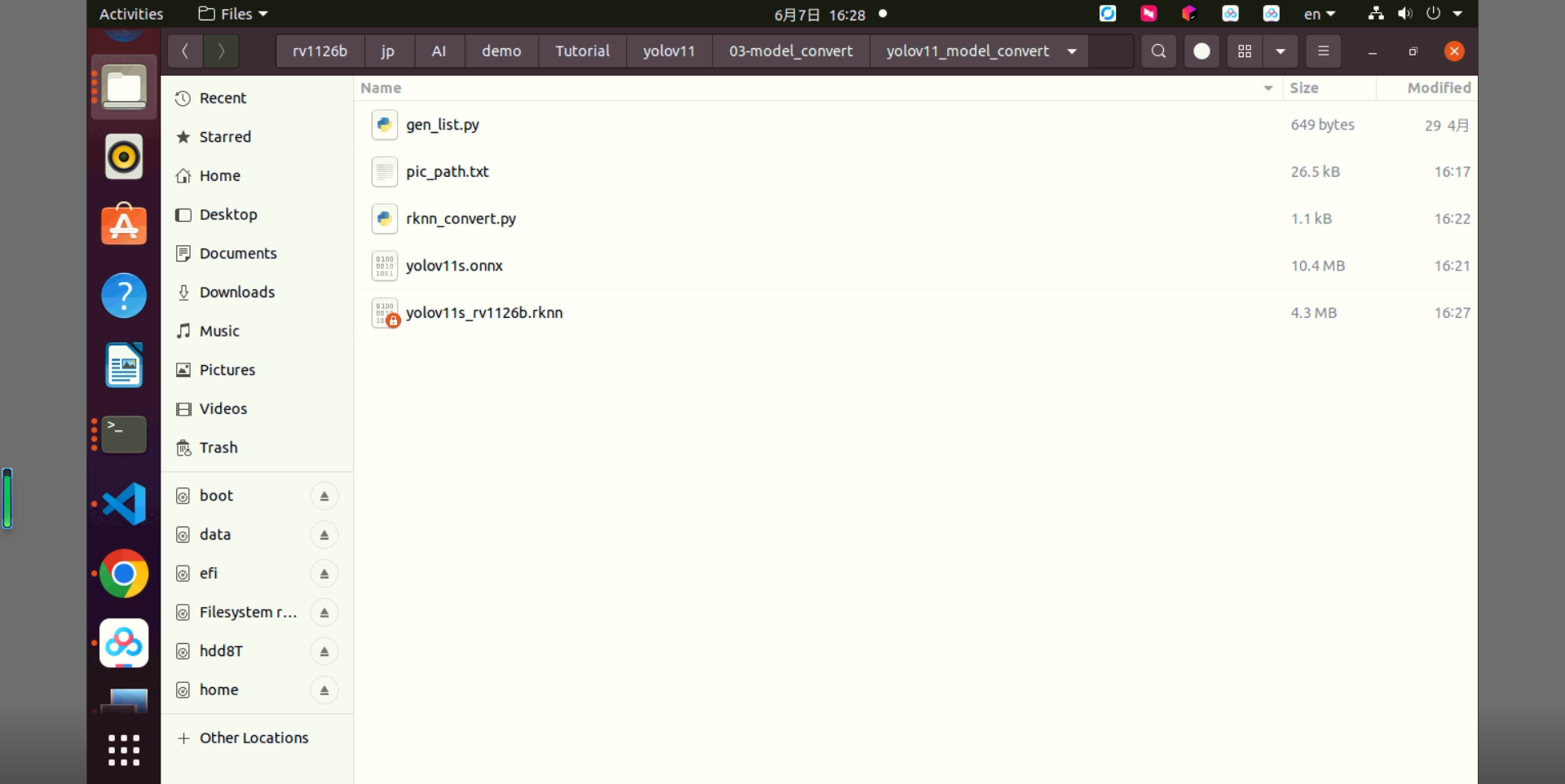
Figure4-6 Generated yolov11s_rv1126b.rknn file after conversion.

5. YOLOv11 Model Deployment

5.1 Deployment Example Description

This section explains how to deploy the YOLOv11 model to the RV1126B board. The trained model in this document is a simple sample model for workflow explanation, and its accuracy is not guaranteed.

5.2 Preparation

5.2.1 Hardware Preparation

Prepare the RV1126B board, a Type-C data cable, and a LAN cable. Use MobaXterm to log in to the RV1126B board through SSH. Refer to the getting-started guide for details.

The topology for LAN connection is shown below.

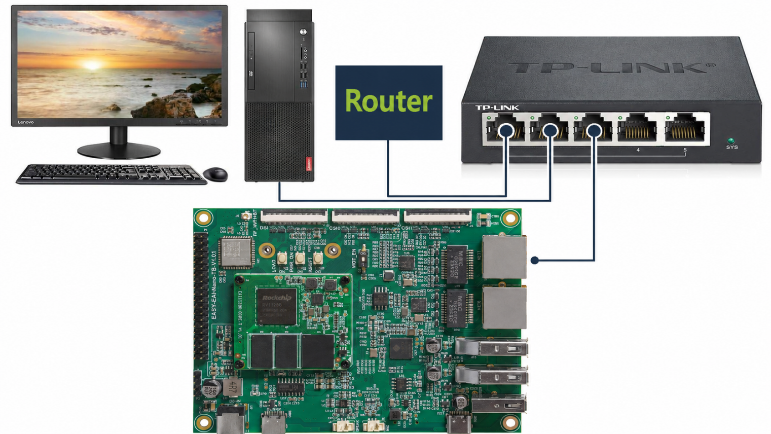
Figure5-1 LAN topology connecting the PC, router, and RV1126B board.

The Type-C serial connection method is shown below.

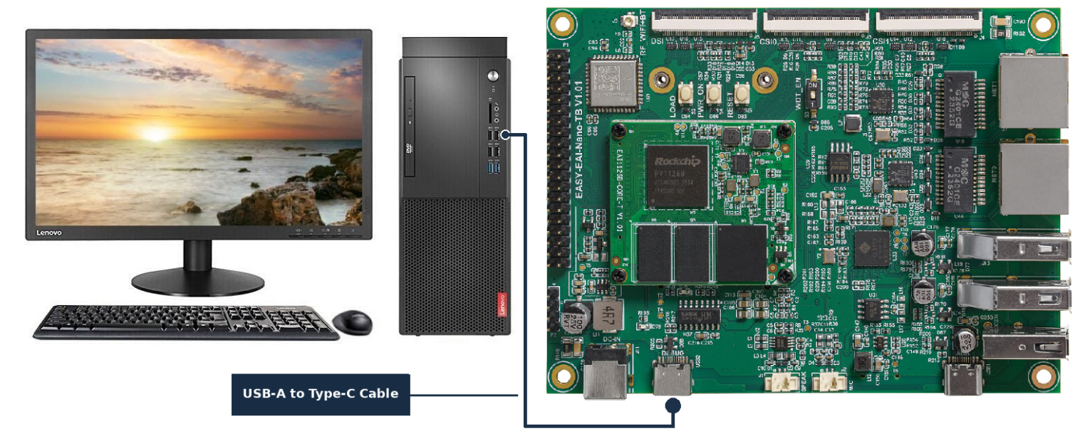
Figure5-2 Connection method between the PC and RV1126B board using a Type-C serial cable.

5.2.2 Prepare the Development Environment

If this is your first time using the guide, refer to the getting-started guide and set up the compilation environment according to the described steps.

Run run.sh on the Ubuntu system on the PC side to enter the RV1126B compilation environment.

cd ~/develop_environment
./run.sh 2204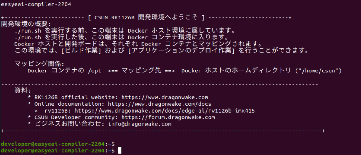

Figure5-3 Startup screen after entering the RV1126B Docker development environment.

5.3 Build the Sample Program

After moving the downloaded package to the RV1126B Docker development environment, extract it with the following commands:

cd /opt/linuxshare/work/rv1126b/jp/AI/demo/Tutorial/yolov11/04-AI_deploy
tar -xJf yolov11_detect_C_demo.tar.xz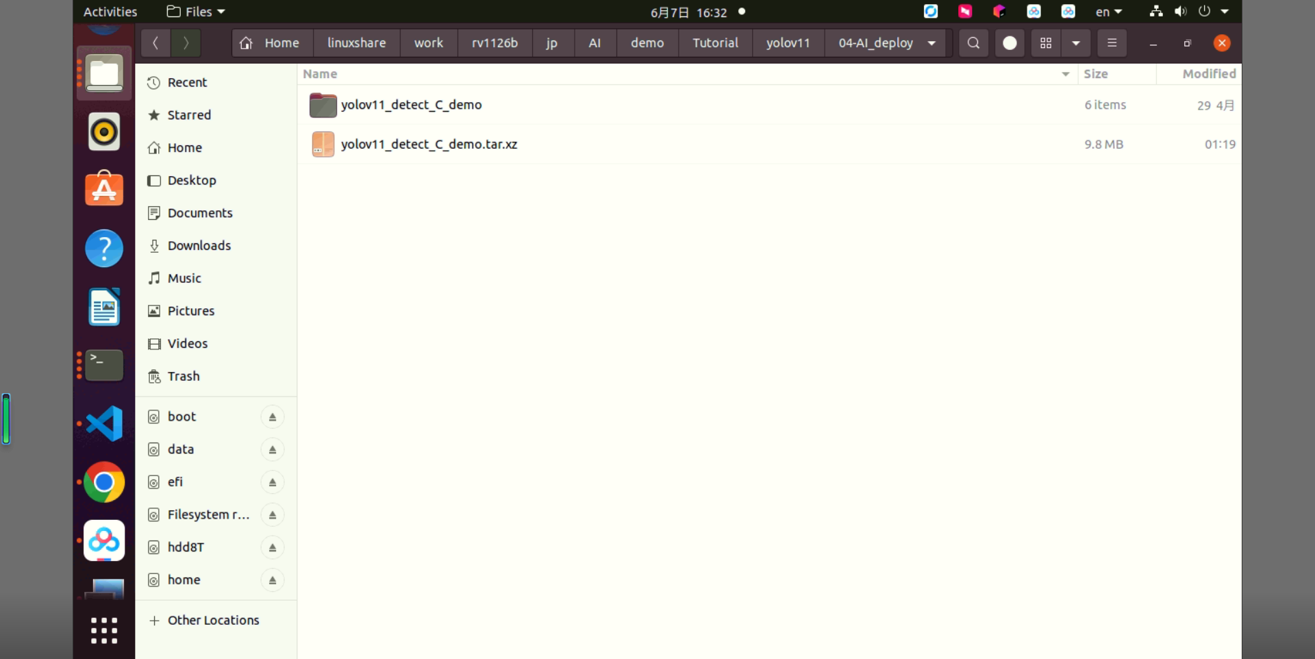

Figure5-4 Directory structure after extracting yolov11_detect_C_demo.

Enter the extracted sample program directory in the RV1126B Docker development environment and build it.

sudo mount -t nfs -o vers=3,proto=tcp,mountproto=tcp,nolock,retrans=5,timeo=5 192.168.11.85:/ /mnt
cd /opt/linuxshare/work/rv1126b/jp/AI/demo/Tutorial/yolov11/04-AI_deploy/yolov11_detect_C_demo/
./build.sh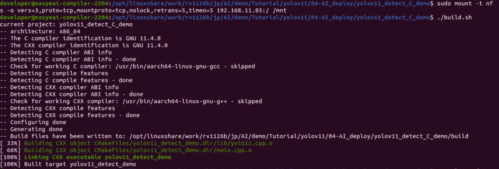

Figure5-5 Terminal output when building the YOLOv11 C demo.

After the build succeeds, copy yolov11_detect_demo_release/ to the /userdata directory on the RV1126B board.

cp yolov11_detect_demo_release/ /mnt/userdata/ -rf

5.4 Run the YOLOv11 Model on the Development Board

Enter the board shell through serial debugging or SSH, then move to the deployment directory of the sample program.

cd /userdata/yolov11_detect_demo_release

Run the sample program as follows:

chmod 777 yolov11_detect_demo
./yolov11_detect_demo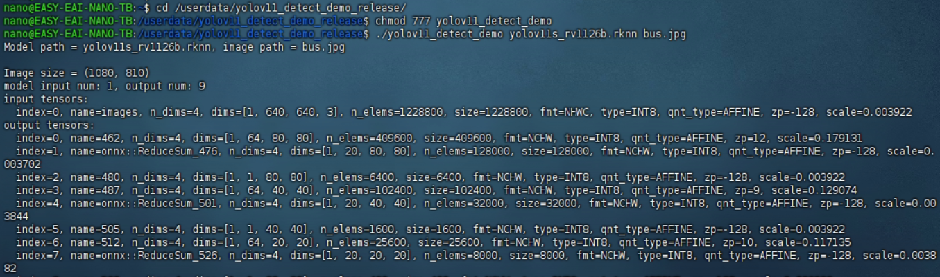

Figure5-6 Log from running the YOLOv11 demo on the RV1126B board.

The algorithm execution time is approximately 40 ms.

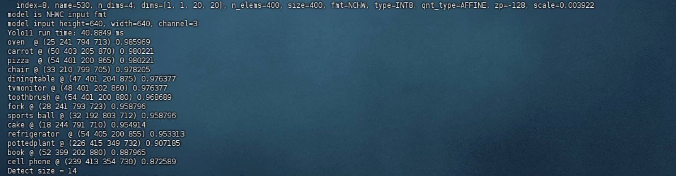
Figure5-7 Algorithm execution time log on the board.

The result image can be obtained from the RV1126B compilation environment with the following command:

cp /mnt/userdata/yolov11_detect_demo_release/result.jpg .

Figure5-8 Command for copying the inference result image from the board to the PC.

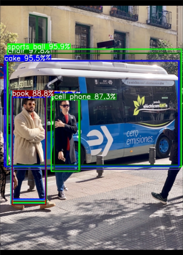
Figure5-9 YOLOv11 object detection result image generated on the RV1126B board.

The YOLOv11 object detection sample has now been successfully executed on the board.